Introduction

Over the next two weeks, we will be learning the basics of Python, like any other language, Python has its own complexities. We won't be able to cover all imaginable topics in this course, but we will cover the basics. The goal of this course is to give you a solid foundation in Python, so that you can continue to learn on your own.

• Setup
• Starting Out
• Control Flow
• Data Structures
• Functions And Classes

This course is going to be a bit more experimental than other courses offered by the IMPRS. Instead of being a full intensity course (half-) day course, we're going to meet for 90 minutes twice a week for two weeks. This will give you more time to work on the exercises and to ask questions.

Instead of simply being a lecture, this course is going to be exercise driven. This means that every session will start with the solution of the previous session's exercises. After that, we will introduce new concepts and give you new exercises to work on. We will then start to solve these exercises together in the session, and the remaining exercises will be for you to solve on your own (which we will then review in the next session).

We will touch the terminal a bit for this course, but we will not go into too much detail. If you want to learn more about the terminal, it is recommended for you to take the Bash course offered by the IMPRS.

To help you through the terminal parts of this course a cheat sheet is provided in the appendix via the Bash Cheat Sheet and Git Cheat Sheet. The Git cheat sheet is only applicable if you are using the Git repository for the exercises (recommended for people with Git experienced, or who have attended the Git 101 or Git 102 course).

After every session, you are able to give feedback on the course, this feedback can be anonymous or not, it is up to you. The feedback form can be found [here]. (It is not mandatory to give feedback, but it is appreciated, it allows us to improve the course.)

Code Snippets

In this book we will have a lot of code snippets, these snippets will be formatted like this:

print("Hello World!")

The expected output from a print statement will be formatted like this:

# > Hello World!

Setup

We will be using Python 3.11 for this course. We will be installing a host of tools to help us with our development process.

These include:

• homebrew (macOS only)
• pyenv
• Python 3.11
• micromamba
• Visual Studio Code
• pipx (optional)
• poetry (optional)

Homebrew

Homebrew is a package manager for macOS. It allows us to install software that is not included in the base macOS install or that is not available via the App Store.

It enables us to install software via the command line, and instead of having to search for a download link, we can simply invoke the following command:

brew install <package>

Homebrew will then download the package and install it for us, it even takes care of dependencies and allows us to install applications that require a GUI.

Installing Homebrew

To install Homebrew, simply open a terminal and paste the following command:

/bin/bash -c "$(curl -fsSL https://raw.githubusercontent.com/Homebrew/install/HEAD/install.sh)"

This will download and install Homebrew for you.

You will be asked to enter your password, as Homebrew needs to be installed in a system directory.

Once the installation is complete, you can verify that it was successful by running the following command:

brew --version

If an error message is displayed, please try to restart your terminal and try again.

Installing packages with Homebrew

To install a package with Homebrew, simply run the following command:

brew install <package>

To update a package, run the following command:

brew upgrade <package>

To update all packages, run the following command:

brew upgrade

To uninstall a package, run the following command:

brew uninstall <package>

Troubleshooting

If you encounter any issues with Homebrew, please refer to the Troubleshooting.

You can also use the brew doctor command to check for common issues.

pyenv

pyenv is a tool that allows us to install and manage multiple versions of Python on our system.

This is especially useful if you are working on multiple projects that require different versions of Python, as python versions are not backwards compatible.

Installing pyenv

To install pyenv, simply run the following command:

brew install pyenv

If you are able to run the pyenv command, you have successfully installed pyenv, otherwise please refer to the Configuring the shell section.

Configuring the shell

If you are unable to run the pyenv command, you will need to configure your shell to use pyenv.

Note: Between macOS 10.15 and 11.0, Apple changed the default shell from bash to zsh. If you are using macOS 10.15 or later, you will need to configure zsh instead of bash. To check which shell you are using, run the following command: ps -o comm= $$

Once you have added the lines to your shell configuration file, you will need to restart your terminal.

Depending on the shell you are using, you will need to add the following lines to your shell configuration file:

Bash

echo 'export PYENV_ROOT="$HOME/.pyenv"' >>~/.bashrc
echo 'command -v pyenv >/dev/null || export PATH="$PYENV_ROOT/bin:$PATH"' >>~/.bashrc
echo 'eval "$(pyenv init -)"' >>~/.bashrc

BASH_PROFILE=0

if [ -e ~/.bash_profile ]; then
  echo 'export PYENV_ROOT="$HOME/.pyenv"' >>~/.bash_profile
  echo 'command -v pyenv >/dev/null || export PATH="$PYENV_ROOT/bin:$PATH"' >>~/.bash_profile
  echo 'eval "$(pyenv init -)"' >>~/.bash_profile
    BASH_PROFILE=1
fi

if [ -e ~/.profile ] && [ $BASH_PROFILE -eq 0 ]; then
  echo 'export PYENV_ROOT="$HOME/.pyenv"' >>~/.profile
  echo 'command -v pyenv >/dev/null || export PATH="$PYENV_ROOT/bin:$PATH"' >>~/.profile
  echo 'eval "$(pyenv init -)"' >>~/.profile
fi

Zsh

echo 'export PYENV_ROOT="$HOME/.pyenv"' >>~/.zshrc
echo 'command -v pyenv >/dev/null || export PATH="$PYENV_ROOT/bin:$PATH"' >>~/.zshrc
echo 'eval "$(pyenv init -)"' >>~/.zshrc

ZPROFILE=0

if [ -e ~/.zprofile ]; then
  echo 'export PYENV_ROOT="$HOME/.pyenv"' >>~/.zprofile
  echo 'command -v pyenv >/dev/null || export PATH="$PYENV_ROOT/bin:$PATH"' >>~/.zprofile
  echo 'eval "$(pyenv init -)"' >>~/.zprofile
  ZPROFILE=1
fi

if [ -e ~/.zlogin ] && [ $ZPROFILE -eq 0 ]; then
  echo 'export PYENV_ROOT="$HOME/.pyenv"' >>~/.zlogin
  echo 'command -v pyenv >/dev/null || export PATH="$PYENV_ROOT/bin:$PATH"' >>~/.zlogin
  echo 'eval "$(pyenv init -)"' >>~/.zlogin
fi

Installing Python with pyenv

To install Python with pyenv, simply run the following command:

pyenv install <version>

You can list all available versions of Python by running the following command:

pyenv install --list

We will install the latest version of Python 3.11, to find out the latest version, run pyenv install --list, then scroll through the list until you find the latest version of Python 3.11. (simply called 3.11.X, chose the version where X is the highest number, do not choose versions that have rc, b, dev, or a in their name)

pyenv install "$(pyenv install --list | grep -e '^[[:space:]]*3.11' | tail -n 1 | xargs)"

Once the installation is complete, you can verify that it was successful by running the following command:

pyenv versions

This will list all installed versions of Python, you should see the version you just installed.

Using Python with pyenv

To use a specific version of Python, simply run the following command:

pyenv global <version>

This will set the specified version of Python as the default version, in any new terminal window. You can verify that it was successful by running the following command:

python --version

This will print the version of Python that is currently being used.

Using Python with pyenv in VSCode

To use a specific version of Python in VSCode, you will need to install the Python extension.

Once the extension is installed, you will need to configure it to use the version of Python you want.

To do this, open the command palette (by pressing cmd + shift + p), then search for Python: Select Interpreter, then select the version of Python you want to use. You can verify that it was successful by running the following command in the VSCode terminal:

python --version

The pyenv version will be recommended by default, but you can also select other versions of Python that are installed on your system. You can verify that you selected the correct version by looking at the path you're selecting, it should be something like /Users/<username>/.pyenv/versions/<version>/bin/python or /Users/<username>/.pyenv/shims/python3.

Installing micromamba

micromamba is a lightweight version of mamba, which is a lightweight version of conda. micromamba is a package manager for Python, which allows you to install Python packages.

There are a multitude of package managers for Python, the data-science community has mostly converged on using conda/mamba for managing Python packages, while the rest of the Python community has mostly converged on using pip/poetry for managing Python packages.

We will be using micromamba to install Python packages, but you can also use pip/poetry if you prefer.

Installing micromamba with Homebrew

To install micromamba with Homebrew, simply run the following command:

brew install micromamba

Installing pipx

pipx is a tool that allows you to install Python packages globally, without polluting your system Python installation, this is important because you don't want to install Python packages globally with pip, as this can cause issues with other Python applications on your system.

Installing pipx with Homebrew

To install pipx with Homebrew, simply run the following command:

brew install pipx

You can then install Python packages globally with pipx, for example:

pipx install poetry

Installing poetry

poetry is a tool that allows you to manage Python packages, it is similar to pip, but it is more modern and has more features.

Installing poetry with Homebrew

To install poetry with Homebrew, simply run the following command:

brew install poetry

Installing VSCode

VSCode is a popular code editor which we will be using for this course, if you prefer to use a different code editor, you can skip this section, but be aware that sections in this course that are specific to VSCode will not be applicable to you. (These sections will be clearly marked)

Installing VSCode with Homebrew

To install VSCode with Homebrew, simply run the following command:

brew install --cask visual-studio-code

Installing VSCode via the website

You can also install VSCode by downloading it from the VSCode website.

Installing VSCode extensions

VSCode extensions are plugins that add additional functionality to VSCode, we will be installing a few extensions that are useful for Python development. You can install extensions by searching for them in the VSCode extensions tab, or by running the following command:

code --install-extension <extension>

Installing the Python extension

The Python extension is the most important extension for Python development, it adds a lot of useful features to VSCode, such as linting, debugging, and code completion. To install it, simply run the following command:

code --install-extension ms-python.python

Note: You can also install the Python extension by searching for it in the VSCode extensions tab.

Setup - Windows

To follow this course, you will need to install a few programs. This page will guide you through the installation process. We will be using the following programs:

• pyenv
• Python 3.11
• micromamba
• Visual Studio Code

These installation instructions require you to open the powershell as an administrator.

Installing pyenv

For more detailed explanation, please refer to the pyenv installation instructions.

To install pyenv, run the following command in the powershell:

Set-ExecutionPolicy -ExecutionPolicy RemoteSigned -Scope LocalMachine

Invoke-WebRequest -UseBasicParsing -Uri "https://raw.githubusercontent.com/pyenv-win/pyenv-win/master/pyenv-win/install-pyenv-win.ps1" -OutFile "./install-pyenv-win.ps1"; &"./install-pyenv-win.ps1"

Installing Python with pyenv

For more detailed explanation, please refer to the Python installation instructions.

To install Python 3.11, run the following command in the powershell:

pyenv install 3.11.X

We will install the latest version of Python 3.11. To find out the latest version, run pyenv install --list and look for the latest version of Python 3.11.

Installing micromamba

For more detailed explanation, please refer to the micromamba installation instructions.

To install micromamba, run the following command in the powershell:

Invoke-Webrequest -URI https://micro.mamba.pm/api/micromamba/win-64/latest -OutFile micromamba.tar.bz2

tar xf micromamba.tar.bz2

.\micromamba.exe --help

To install the latest version of micromamba, you first need to create a new directory for micromamba, here we will create a directory called micromamba in the root of the C: drive. (You can also create the directory somewhere else, but you will need to adjust the path in the following commands.)

mkdir C:\micromamba

To then install the latest version of micromamba, run the following command in the powershell:

$Env:MAMBA_ROOT_PREFIX="C:\micromamba"
.\micromamba.exe shell hook -s powershell | Out-String | Invoke-Expression

Then, initialise the powershell to recognise micromamba:

micromamba shell init -s powershell -p C:\micromamba

Installing Visual Studio Code

For more detailed explanation, please refer to the Visual Studio Code installation instructions.

To install Visual Studio Code head over to the Visual Studio Code website and download the installer. Then, run the installer and follow the instructions.

Starting Out - The Fundamentals

The goal of this section is to introduce the fundamentals of Python. We will cover the following topics:

• Program Structure
• Comments
• Variables
• Expressions
• Operators
• Primitive Types
• Functions and Methods
  • Common Built-in Functions
  • Common Built-in Methods

Program Structure

A Python program is a sequence of statements. A statement is a line of code that performs some action. For example, the following program prints the string "Hello, World!" to the console:

print("Hello, World!")

Programs are executed from top to bottom. The first statement in a program is executed first, followed by the second statement, and so on. In the above example, the print statement is the only statement in the program, so it is executed first.

Python programs are whitespace sensitive, meaning that the indentation of a line of code is important. The indentation of a like is the number of spaces at the beginning of the line. The number of spaces used for indentation must be the same across all lines of code, we choose to use 4 spaces for indentation. This means that if we talk about an indentation of 2, we mean 8 spaces.

Programs are structured using indentation. Indentation is the number of spaces at the beginning of a line. Indentation is used during control flow statements, such as if statements and for loops. We will cover control flow in a later section.

An example of indentation is shown below:

if True:
    print("Hello, World!")

Comments

Comments are lines of code that are ignored by the Python interpreter. Comments are used to explain what a line (or multiple lines) of code does. While other languages like C have a distinction between single line comments and multi line comments, Python only has a single type of comment. Comments are created by starting a line with a # character. Everything after the # character is ignored by the Python interpreter.

# This is a comment
print("Hello, World!")  # This is also a comment
# print("This line is commented out") <- this will not be executed

Lines that are comments are usually grayed out in IDEs and text editors.

We will use comments throughout this course to explain what a line of code does or to explain the task at hand that you need to solve in an exercise.

Multi Line Comments

Python does not have a multi line comment syntax. However, there is a trick to create multi line comments. Multi line comments are created by using a multi line string. A multi line string is a string that spans multiple lines. Multi line strings are created by using three double quotes (""") or three single quotes ('''). The following example shows how to create a multi line string:

"""
This is a multi line string.
This is the second line of the string.
This is the third line of the string.
"""

When putting a multi line string at the beginning of a file, it is interpreted as a multi line comment. These comments are used throughout the exercises in this course to explain the task at hand.

These comments are often referred to as docstrings, because they are used to document a program or function as a whole, instead of a single line of code.

Note: Multi line comments are also valid in other places in a Python program, they are also used to create documentation for functions and classes. We will cover functions and classes in a later section.

def my_function():
    """This is the documentation of my_function"""
    pass
    
print(my_function.__doc__)
# > This is the documentation of my_function 

Variables

Variables are used to store values in memory. Variables are created by assigning a value to a name. The name of a variable can be chosen freely, but it must follow the following rules:

• The name must start with a letter or an underscore (_)
• The name can only contain letters, numbers and underscores (_)
• The name cannot be a reserved keyword
• The name cannot contain spaces
• The name cannot start with a number
• The name is case sensitive

Additionally in this course, we will enforce the following rules:

• The name must be descriptive
• The name must be in snake_case (all lowercase, words separated by underscores)
• The name must be in English
• Constants must be in UPPER_SNAKE_CASE (all uppercase, words separated by underscores)
  • A constant is a variable that is not supposed to change during the execution of a program

Variables are created by assigning a value to a name using the assignment operator (=). The assignment operator is a binary operator, meaning that it takes two operands. The left operand is the name of the variable, the right operand is the value that is assigned to the variable.

The following example shows how to create a variable:

my_variable = 42
print(my_variable)
# > 42

The above example creates a variable named my_variable and assigns the value 42 to it. The value of a variable can be changed by assigning a new value to it.

my_variable = 42
print(my_variable)
# > 42

my_variable = 43
print(my_variable)
# > 43

Variables can be used in expressions. The value of the variable is used in the expression. The following example shows a variable being used in an expression:

my_variable = 42
print(my_variable + 1)
# > 43

Expressions

Expressions are combinations of values, variables and operators. Expressions are evaluated by the Python interpreter. An expression can be a single value, a variable or a combination of values, variables and operators.

The following example shows a single value being used as an expression:

print(42)
# > 42

The following example shows a variable being used as an expression:

my_variable = 42
print(my_variable)
# > 42

The following example shows a combination of values, variables and operators being used as an expression:

print(42 + 1)
# > 43

Operators

Operators are used to perform operations on values and variables. Operators are used in expressions, they are used to combine values, variables and other operators. Operators can be used to perform arithmetic operations, comparison and to combine values.

There are different types of operators that are supported by Python, these include:

• Arithmetic operators
  • Addition (+)
  • Subtraction (-)
  • Multiplication (*)
  • Division (/)
  • Floor division (//)
  • Modulo (%)
  • Exponentiation (**)
  • Negation (-)
• Comparison operators
  • Equal to (==)
  • Not equal to (!=)
  • Greater than (>)
  • Greater than or equal to (>=)
  • Less than (<)
  • Less than or equal to (<=)
• Logical operators
  • Logical AND (and)
  • Logical OR (or)
  • Logical NOT (not)
• Assignment operators
  • Assignment (=)
  • Expression and assignment (+=, -=, *=, /=, //=, %=, **=, &=, |=, ^=, <<=, >>=)
  • Walrus operator (:=)
• Identity operators
  • Identity (is)
  • Not identity (is not)
• Membership operators
  • Membership (in)
  • Not membership (not in)
• Bitwise operators (we will not cover these in this course, they only here for completeness)
  • Bitwise AND (&)
  • Bitwise OR (|)
  • Bitwise XOR (^)
  • Bitwise NOT (~)
  • Bitwise left shift (<<)
  • Bitwise right shift (>>)

Arithmetic operators

Arithmetic operators are used to perform arithmetic operations on values and variables, they obey the rules of mathematics, this means that / binds stronger than +. Meaning that 3 + 4 / 2 is evaluated as 3 + (4 / 2).

The following example shows how to use arithmetic operators:

print(3 + 4 * 5)
# > 23

Comparison operators

Comparison operators are used to compare values and variables. They return a boolean value (True or False).

The following example shows how to use comparison operators:

print(3 > 4)
# > False

Logical operators

Logical operators are used to combine boolean values. They return a boolean value (True or False). Logical operators are used to combine boolean values, they are used to check if multiple conditions are met.

The following example shows how to use logical operators:

print(True and False)
# > False

print(bool(0))
# > False
print(bool(0.0))
# > False
print(bool(''))
# > False
print(bool([]))
# > False
print(bool({}))
# > False
print(bool(None))
# > False

print(bool(1))
# > True
print(bool(0.1))
# > True
print(bool(' '))
# > True
print(bool([1]))
# > True
print(bool({1: 1}))
# > True

Truth tables

Logical operators can be represented using truth tables. Truth tables are used to show the result of a logical operator when combining two boolean values.

The following truth table shows the result of the logical AND operator (and):

The following truth table shows the result of the logical OR operator (or):

The following truth table shows the result of the logical NOT operator (not):

Assignment operators

Assignment operators are used to assign values to variables. Assignment operators are used to assign values to variables in expressions.

There are different types of assignment operators, these include:

• Simple assignment (=)
• Expression and assignment (+=, -=, *=, /=, //=, %=, **=, &=, |=, ^=, <<=, >>=)
• Walrus operator (:=)

The simple assignment operator (=) is used to assign a value to a variable. The following example shows how to use the simple assignment operator:

my_variable = 42
print(my_variable)
# > 42

The expression and assignment operators are used to combine an expression and an assignment. The following example shows how to use the expression and assignment operators:

my_variable = 42
my_variable += 1
print(my_variable)
# > 43

# equivalent to:
my_variable = 42
my_variable = my_variable + 1
print(my_variable)
# > 43

The variable X= expression assignment is equivalent to variable = variable X expression, where X is one of the following operators: +, -, *, /, //, %, **, &, |, ^, <<, >>.

The walrus operator (:=) is used to assign a value to a variable and return the value. It is only used in advanced circumstances, but can be used to propagate a value in a chain of function calls.

The following example shows how to use the walrus operator:

y = (x := 42)
print(x)
# > 42
print(y)
# > 42

Identity operators

Identity operators are used to compare the identity of two objects, we won't cover what identity means in this course, but you can read more about it here.

For now it is enough to know that if we want to check if a value is None, we can use the identity operator is.

Membership operators

Membership operators are used to check if a value is a member of a collection. We will cover collections in the data structures part of this course.

For now it is enough to know that if we want to check if a value is in a list, we can use the membership operator in. We can also check if a substring is in a string.

The following example shows how to use the membership operator:

print(1 in [1, 2, 3])
# > True
print('a' in 'abc')
# > True

Primitive Types

In Python, there are different types of values, we will get into more detail about these types in the data structures chapter.

Primitive types are the most basic types of values, they are the building blocks of all other types of values. They are called primitive types because they are not built using other types of values.

Python supports the following primitive types:

• Numeric types
  • int
  • float
  • complex
• Strings
• Booleans
• None

Numeric types

Numeric types are used to represent numbers. Python supports three numeric types: int, float and complex. The int type is used to represent integers, the float type is used to represent floating point numbers, and are very heavily used. The complex type is used to represent complex numbers, which are not used very often.

The following example shows how to use numeric types:

print(42)
# > 42
print(42.0)
# > 42.0
print(42 + 0j)
# > (42+0j)

Each numeric type has their respective functions, which can be used to convert a value to that type. The following example shows how to convert a string to a numeric type:

value = "42"
print(int(value))
# > 42
print(float(value))
# > 42.0
print(complex(value))
# > (42+0j)

Strings

Strings are used to represent text. You can construct a string by surrounding a sequence of characters with either single quotes (') or double quotes ("). The following example shows how to construct a string:

print('Hello World!')
# > Hello World!
print("Hello World!")
# > Hello World!

You cannot mix single quotes and double quotes, the following example shows what happens when you try to do that:

print('Hello World!")
# > SyntaxError: EOL while scanning string literal

You cannot use a new line in a string, the following example shows what happens when you try to do that:

print('Hello
World!')
# > SyntaxError: EOL while scanning string literal

To be able to use a newline in a string, you can either use the \n escape sequence, or use a multiline string. The following example shows how to use the \n escape sequence:

print('Hello\nWorld!')
# > Hello
# > World!

The following example shows how to use a multiline string:

print('''Hello
World!''')
# > Hello
# > World!

You can use some of the arithmetic operators with strings, the following example shows how to use the + operator with strings:

print('Hello' + 'World!')
# > HelloWorld!

You can also use the * operator with strings, the following example shows how to use the * operator with strings:

print('Hello' * 3)
# > HelloHelloHello

You can also include values in strings using f-strings, the following example shows how to use f-strings:

name = 'John'
print(f'Hello {name}!')
# > Hello John!

Booleans

Booleans are used to represent truth values. Booleans can only have two values, True and False.

The following example shows how to use booleans:

print(True)
# > True
print(False)
# > False

You can produce booleans using comparison operators, the following example shows how to use comparison operators:

print(1 == 1)
# > True
print(1 != 1)
# > False

None

None expresses the absence of a value. This value is usually returned by functions that either don't return anything, or only return something under certain conditions.

The following example shows how to use None:

print(None)
# > None

Methods and Functions

We won't get into too much detail about methods and functions in this chapter, as we will get into more detail about them in the functions chapter.

Functions are pieces of code that can be reused, they are used to perform a specific task. Functions can take inputs, and can return outputs.

There are two types of functions, methods and functions. Methods are functions that are attached to an object, and are called using the dot notation. Functions are not attached to an object, and are called using their name.

The following example shows how to call a method:

print('Hello World!'.lower())
# > hello world!

The following example shows how to call a function:

print(len('Hello World!'))
# > 12

Built-in Functions

Python comes with a lot of built-in functions and methods with can be used to perform a wide variety of tasks. These include:

You can find a full list of built-in functions here.

print

The print function is used to print a value to the console. The following example shows how to use the print function:

print('Hello World!')
# > Hello World!

input

The input function is used to get input from the user. The following example shows how to use the input function:

name = input('Enter your name: ')
print(f'Hello {name}!')
# > Enter your name: John
# > Hello John!

type

The type function is used to get the type of a value. The following example shows how to use the type function:

print(type(1))
# > <class 'int'>
print(type(1.0))
# > <class 'float'>
print(type('Hello World!'))
# > <class 'str'>
print(type(True))
# > <class 'bool'>
print(type(None))
# > <class 'NoneType'>

int, float, str, bool

The int, float, str, and bool functions are used to convert values to integers, floats, strings, and booleans.

The following example shows how to use the int function:

print(int(1.0))
# > 1
print(int('1'))
# > 1
print(int(True))
# > 1
print(int(False))
# > 0

The following example shows how to use the float function:

print(float(1))
# > 1.0
print(float('1'))
# > 1.0
print(float(True))
# > 1.0
print(float(False))
# > 0.0

The following example shows how to use the str function:

print(str(1))
# > '1'
print(str(1.0))
# > '1.0'
print(str(True))
# > 'True'
print(str(False))
# > 'False'

The following example shows how to use the bool function:

print(bool(1))
# > True
print(bool(1.0))
# > True
print(bool('Hello World!'))
# > True
print(bool(None))
# > False

len

The len function is used to get the length of a value. The following example shows how to use the len function:

print(len('Hello World!'))
# > 12

open

The open function is used to open a file. The following example shows how to use the open function:

file = open('file.txt', 'r')
print(file.read())
# > Hello World!
file.close()

help

The help function is used to get help on a function. The following example shows how to use the help function:

help(print)
# > Help on built-in function print in module builtins:
# >
# > print(...)
# >     print(value, ..., sep=' ', end='\n', file=sys.stdout, flush=False)
# >
# >     Prints the values to a stream, or to sys.stdout by default.
# >     Optional keyword arguments:
# >     file:  a file-like object (stream); defaults to the current sys.stdout.
# >     sep:   string inserted between values, default a space.
# >     end:   string appended after the last value, default a newline.
# >     flush: whether to forcibly flush the stream.

eval

The eval function is used to evaluate a string as a Python expression. The following example shows how to use the eval function:

print(eval('1 + 1'))
# > 2

Note: The eval function is dangerous, and should not be used unless you know what you are doing.

Built-in Methods

str

The str has a multitude of methods, some of which are shown below. You can find a full list of methods on the Python documentation.

lower

The lower method is used to convert a string to lowercase. The following example shows how to use the lower method:

print('Hello World!'.lower())
# > hello world!

upper

The upper method is used to convert a string to uppercase. The following example shows how to use the upper method:

print('Hello World!'.upper())
# > HELLO WORLD!

title

The title method is used to convert a string to title case. The following example shows how to use the title method:

print('hello world!'.title())
# > Hello World!

capitalize

The capitalize method is used to capitalize the first letter of a string. The following example shows how to use the capitalize method:

print('hello world!'.capitalize())
# > Hello world!

strip

The strip method is used to remove whitespace from the beginning and end of a string. The following example shows how to use the strip method:

print('   Hello World!   '.strip())
# > Hello World!

lstrip

The lstrip method is used to remove whitespace from the beginning of a string. The following example shows how to use the lstrip method:

print('   Hello World!   '.lstrip())
# > Hello World!   

rstrip

The rstrip method is used to remove whitespace from the end of a string. The following example shows how to use the rstrip method:

print('   Hello World!   '.rstrip())
# >    Hello World!

replace

The replace method is used to replace a substring with another substring. The following example shows how to use the replace method:

print('Hello World!'.replace('World', 'Universe'))
# > Hello Universe!

split

The split method is used to split a string into a list of substrings. The following example shows how to use the split method:

print('Hello World!'.split())
# > ['Hello', 'World!']

join

The join method is used to join a list of substrings into a string. The following example shows how to use the join method:

print(' '.join(['Hello', 'World!']))
# > Hello World!

startswith

The startswith method is used to check if a string starts with a substring. The following example shows how to use the startswith method:

print('Hello World!'.startswith('Hello'))
# > True

endswith

The endswith method is used to check if a string ends with a substring. The following example shows how to use the endswith method:

print('Hello World!'.endswith('World!'))
# > True

find

The find method is used to find the index of a substring. The following example shows how to use the find method:

print('Hello World!'.find('World'))
# > 6

removeprefix

The removeprefix method is used to remove a prefix from a string. The following example shows how to use the removeprefix method:

print('Hello World!'.removeprefix('Hello '))
# > World!

removesuffix

The removesuffix method is used to remove a suffix from a string. The following example shows how to use the removesuffix method:

print('Hello World!'.removesuffix(' World!'))
# > Hello

Control Flow

The goal of this section is to introduce the control flow statements in Python. We will cover the following topics:

• Conditionals
• Loops
  • for Loops
  • while Loops
  • break and continue
  • pass Statements
  • range() Function
• match Statements

Conditionals

Conditionals are used to control the flow of a program. They allow us to execute certain blocks of code only if certain conditions are met. In Python a conditional is created using the if statement. The if statement is followed by an expression which is evaluated to a boolean value. If the expression evaluates to True then the code block following the if statement is executed. If the expression evaluates to False then the code block is skipped.

It is important to note that the code block following the if statement is indented. This is how Python knows which block of code is associated with the if statement. The code block is indented by 4 spaces by convention and ends when the indentation returns to the previous level.

if True:
    print("This code block will be executed")
    # > This code block will be executed

    print("This code block will also be executed")
    # > This code block will also be executed

print("This code block will be executed as well")
# > This code block will be executed as well

if False:
    print("This code block will not be executed")

print("This code block will be executed as well")
# > This code block will be executed as well

if 1 == 1:
    print("This code block will be executed")
    # > This code block will be executed

if 1 == 2:
    print("This code block will not be executed")

The if statement can be followed by an else statement. The else statement is followed by a code block that will be executed if the expression in the if statement evaluates to False.

if True:
    print("This code block will be executed")
    # > This code block will be executed
else:
    print("This code block will not be executed")

if False:
    print("This code block will not be executed")
else:
    print("This code block will be executed")
    # > This code block will be executed

The if statement can also be followed by an elif statement. The elif statement is followed by an expression that will be evaluated if the expression in the if statement evaluates to False. If the expression in the elif statement evaluates to True then the code block following the elif statement will be executed. If the expression in the elif statement evaluates to False then the code block following the elif statement will be skipped.

if False:
    print("This code block will not be executed")
elif True:
    print("This code block will be executed")
    # > This code block will be executed
else:
    print("This code block will not be executed")

if False:
    print("This code block will not be executed")
elif False:
    print("This code block will not be executed")
else:
    print("This code block will be executed")
    # > This code block will be executed

The if statement can be followed by any number of elif statements, but an else statement cannot be followed by an elif statement. The else statement must be the last statement in the conditional.

if False:
    print("This code block will not be executed")
elif False:
    print("This code block will not be executed")
elif False:
    print("This code block will not be executed")
else:
    print("This code block will be executed")
    # > This code block will be executed

Loops

Loops are used to execute a block of code multiple times. In Python there are two types of loops: for loops and while loops.

for Loops

for loops are used to iterate over a sequence of values. The sequence can be a list, tuple, string, or any other type of sequence. The for loop will iterate over each value in the sequence and execute the code block following the for loop once for each value in the sequence, the value will be assigned to a variable in the code block to the name chosen in the for loop.

for i in [1, 2, 3]:
    print(i)

# > 1
# > 2
# > 3

for i in (1, 2, 3):
    print(i)

# > 1
# > 2
# > 3

for i in "abc":
    print(i)

# > a
# > b
# > c

The for loop can be followed by an else statement. The else statement is followed by a code block that will be executed once the for loop has finished iterating over the sequence, and no break statement was executed. This is very seldom used.

for i in [1, 2, 3]:
    print(i)
else:
    print("The for loop has finished iterating")

# > 1
# > 2
# > 3
# > The for loop has finished iterating

for i in [1, 2, 3]:
    print(i)
    break
else:
    print("The for loop has finished iterating")

# > 1

while Loops

while loops are used to execute a block of code while a condition is True. The condition is evaluated before each execution of the code block. If the condition evaluates to True then the code block is executed. If the condition evaluates to False then the code block is skipped.

i = 0
while i < 3:
    print(i)
    i += 1

# > 0
# > 1
# > 2

The while loop can be followed by an else statement. The else statement is followed by a code block that will be executed once the while loop has finished iterating, and no break statement was executed. This is very seldom used.

i = 0
while i < 3:
    print(i)
    i += 1
else:
    print("The while loop has finished iterating")

# > 0
# > 1
# > 2
# > The while loop has finished iterating

i = 0
while i < 3:
    print(i)
    i += 1
    break
else:
    print("The while loop has finished iterating")

# > 0

The rule of thumb is: try to use for loops when you know how many times you want to iterate, and use while loops when you don't. (meaning prefer for loops over while loops)

break and continue

break and continue are used to control the flow of a loop. break is used to exit the loop immediately, and the code block following the loop will be executed. continue is used to skip the rest of the code block and continue with the next iteration of the loop.

for i in [1, 2, 3]:
    print(i)
    break

# > 1

for i in [1, 2, 3]:
    print(i)
    continue
    print("This code block will not be executed")

# > 1
# > 2
# > 3

pass

pass is used as a placeholder for code that has not been written yet. It is used to prevent a syntax error when a code block is required but you don't want to write any code in the code block yet.

if True:
    pass
else:
    print("This code block will not be executed")

for i in [1, 2, 3]:
    pass

In more modern versions of Python, ... can be used instead of pass.

if True:
    ...
else:
    print("This code block will not be executed")

for i in [1, 2, 3]:
    ...

range()

The range() function is used to generate a sequence of numbers. It can be used to generate a sequence of numbers from a specified start value to a specified end value. The end value is not included in the sequence. The range function is predominately used in for loops to iterate over a sequence of numbers, or to iterate a specified number of times.

The range function can be called with one, two, or three arguments. If called with one argument, the argument is the end value of the sequence, the start value is assumed to be 0, and the step value is assumed to be 1. If called with two arguments, the first argument is the start value of the sequence, the second argument is the end value of the sequence, and the step value is assumed to be 1. If called with three arguments, the first argument is the start value of the sequence, the second argument is the end value of the sequence, and the third argument is the step value of the sequence.

for i in range(1, 4):
    print(i)

# > 1
# > 2
# > 3

for i in range(3):
    print(i)

# > 0
# > 1
# > 2

for i in range(1, 4, 2):
    print(i)

# > 1
# > 3

for i in range(4, 1, -1):
    print(i)

# > 4
# > 3
# > 2

match Statements

Note: By no means are match statements necessary to learn Python. They are a relatively new feature in Python, and you can skip this section if you want. You can achieve the same results using if statements (we've done so for years and survived!).

match statements are a relatively new feature in Python. They are used to compare a value to a number of patterns and execute code based on which pattern matches the value. match statements are similar to switch statements in other languages.

Each case in a match statement is followed by a pattern and a colon. The code block following the case statement is executed if the value matches the pattern.

There are several types of patterns, these include:

• Literal patterns
• Capture patterns
• Wildcard patterns
• Value patterns
• Group patterns
• Sequence patterns
• Mapping patterns
• Class patterns

Literal Patterns

Literal patterns are used to match a value to a literal value. Literal patterns are written as the literal value.

match 1:
    case 1:
        print("The value is 1")
    case 2:
        print("The value is 2")

# > The value is 1

Capture Patterns

Capture patterns are used to match a value to a variable. Capture patterns are written as a variable name, the variable name _ is invalid, as it is used as a wildcard pattern.

match 1:
    case x:
        print(f"The value is {x}")

# > The value is 1

Wildcard Patterns

Wildcard patterns are used to match any value. Wildcard patterns are written as _.

match 1:
    case _:
        print("The value is 1")

# > The value is 1

Value Patterns

Value patterns are used to match against the value of a variable. Due to conflicts with capture patterns, value patterns are only valid if they contain . (are accessing an attribute of a variable).

from enum import Enum


class Color(Enum):
    RED = 1
    GREEN = 2
    BLUE = 3


color = Color.RED

match color:
    case Color.RED:
        print("The color is red")
    case Color.GREEN:
        print("The color is green")
    case Color.BLUE:
        print("The color is blue")

# > The color is red

Group Patterns

Group patterns are written as (...), they are not required, but can be used to make the code more readable. (They cannot contain a comma, as otherwise they would be interpreted as a sequence pattern)

match 1:
    case (1):
        print("The value is 1")
    case (2):
        print("The value is 2")

# > The value is 1

Sequence Patterns

Sequence patterns are used to match a value to a sequence of values. Sequence patterns are written as [...]. Sequence patterns can nest other patters as elements and use *var to capture the rest of the sequence.

a = [1, 2, 3]

match a:
    case [1, *rest]:
        print(f"The rest of the sequence is {rest}")

# > The rest of the sequence is [2, 3]

match a:
    case [*rest, 3]:
        print(f"The rest of the sequence is {rest}")

# > The rest of the sequence is [1, 2]

match a:
    case [1, *rest, 3]:
        print(f"The rest of the sequence is {rest}")

# > The rest of the sequence is [2]

match a:
    case [1, 2, 3]:
        print("The sequence is [1, 2, 3]")

# > The sequence is [1, 2, 3]

match a:
    case [1, 2, 3, 4]:
        print("The sequence is [1, 2, 3, 4]")
    case [1, 2, 3]:
        print("The sequence is [1, 2, 3]")

# > The sequence is [1, 2, 3]

Sequence patterns can also be used to match tuples, in that case the sequence pattern is written as (...).

a = (1, 2, 3)

match a:
    case (1, *rest):
        print(f"The rest of the sequence is {rest}")

# > The rest of the sequence is (2, 3)

Mapping Patterns

Mapping patterns are used to match a value to a mapping of values. Mapping patterns are written as {...}. Mapping patterns can nest other patters as values and use **var to capture the rest of the mapping.

a = {"a": 1, "b": 2, "c": 3}

match a:
    case {"a": 1, **rest}:
        print(f"The rest of the mapping is {rest}")

# > The rest of the mapping is {'b': 2, 'c': 3}

match a:
    case {"a": 1, **rest, "c": 3}:
        print(f"The rest of the mapping is {rest}")

# > The rest of the mapping is {'b': 2}

match a:
    case {"a": 1, "b": 2, "c": 3, "d": 4}:
        print("The mapping is {'a': 1, 'b': 2, 'c': 3, 'd': 4}")
    case {"a": 1, "b": 2, "c": 3}:
        print("The mapping is {'a': 1, 'b': 2, 'c': 3}")

# > The mapping is {'a': 1, 'b': 2, 'c': 3}

Class Patterns

Class patterns are used to match a value to a class. Class patterns are written as ClassName(...). Class patterns can nest other patters as arguments and use **var to capture the rest of the mapping.

class A:
    pass


a = A()

match a:
    case A():
        print("The value is an instance of A")

# > The value is an instance of A

match 1:
    case int():
        print("The value is an instance of int")
    case float():
        print("The value is an instance of float")

# > The value is an instance of int

Guard Patterns

Guard patterns are used to match a value to a pattern and then check if a condition is true. Guard patterns are written as pattern if condition.

match 1:
    case x if x > 0:
        print(f"The value is {x}")

# > The value is 1

As Patterns

As patterns are used to match a value to a pattern and then capture the value in a variable. As patterns are written as pattern as var.

match 1:
    case x as y:
        print(f"The value is {x}")
        print(f"The value is also {y}")

# > The value is 1
# > The value is also 1

Or Patterns

Or patterns are used to match a value to multiple patterns. Or patterns are written as pattern1 | pattern2.

match 1:
    case 1 | 2:
        print("The value is 1 or 2")

# > The value is 1 or 2

match 2:
    case 1 | 2:
        print("The value is 1 or 2")

# > The value is 1 or 2

Data Structures

In the previous chapters we have talked about primitive data types, such as int, float, bool, str, and None. These are the basic building blocks of any program, but they are not enough to solve most real-world problems. In this chapter we will introduce more complex data types, which are called data structures.

We will cover the following data structures:

• Lists
• Tuples
• Sets
• Dictionaries
• Dataclasses
• Enumerations

Guidance

If you don't know which type of collection to use, here is a simple decision diagram:

flowchart TD
    A[I want to save a list of things]

    A --> B{{ Do my values have a unique key<br/> and associated value? }}
    B -->|No| D{{Do I mainly check if a value is the collection?}}

    D -->|Yes| E{{Are all values unique?}}
    D -->|No| I
    
    E -->|No| I{{Do I only insert values once?}}
    I -->|Yes| J[use <code>tuple</code>]
    I -->|No| C[use <code>list</code>]
    B -->|Yes| L[use <code>dict</code>]
    
    E -->|Yes| M{{Do I need to know the order of the values?}}
    M -->|Yes| C
    M -->|No| G{{Do I only insert values once<br/>and then check against those?}}
    G -->|Yes| H[use <code>frozenset</code>]
    G -->|No| F[use <code>set</code>]

Lists

Lists are an ordered collection of items, they can contain any type of data, and can be modified after creation (they are mutable). Lists allow for duplicate items, they are indexed, and are iterable.

Creating Lists

Lists are created using square brackets [] and items are separated by commas ,.

a = [1, 2, 3, 4, 5]

print(a)
# > [1, 2, 3, 4, 5]

b = [1, 'a', 2, 'b', 3, 'c']
print(b)

Accessing Items

Items in a list can be accessed using their index. They are zero-indexed, meaning the first item is at index 0, the second item is 1, and so on. Indexes can also be negative, where -1 is the last item, -2 is the second to last item, etc.

When indexing out of bounds, an IndexError is raised.

a = [1, 2, 3, 4, 5]

print(a[0])
# > 1

print(a[2])
# > 3

print(a[-1])
# > 5

print(a[-3])
# > 3

print(a[5])
# > IndexError: list index out of range

Slicing

Slicing is a way to get a subset of a list. It is done by specifying a start index, an end index, and a step. The start index is inclusive, the end index is exclusive, and the step is the number of items to skip.

They syntax for slicing is list[start🔚step]. If any of the values are omitted, they default to the following: list[0:len(list):1].

a = [1, 2, 3, 4, 5]

print(a[1:3])  # when omitting the step we can also omit the colon
# > [2, 3]

print(a[1:5:2])
# > [2, 4]

print(a[::2])
# > [1, 3, 5]

print(a[1::2])
# > [2, 4]

print(a[::-1])
# > [5, 4, 3, 2, 1]

Modifying Lists

Lists are mutable, meaning they can be modified after creation. This is done by assigning a new value to an index or a slice.

a = [1, 2, 3, 4, 5]

a[0] = 10
print(a)
# > [10, 2, 3, 4, 5]

a[1:3] = [20, 30]
print(a)
# > [10, 20, 30, 4, 5]

a[1:3] = [40, 50, 60, 70]
print(a)
# > [10, 40, 50, 60, 70, 4, 5]

You can also use methods to modify lists. Some of the most common methods are:

• append(item) - adds an item to the end of the list
• extend(list) - adds all items in the given list to the end of the list
• insert(index, item) - inserts an item at the given index
• remove(item) - removes the first occurrence of the given item
• pop() - removes and returns the last item in the list
• pop(index) - removes and returns the item at the given index
• clear() - removes all items from the list

a = [1, 2, 3, 4, 5]

a.append(6)
print(a)
# > [1, 2, 3, 4, 5, 6]

a.extend([7, 8, 9])
print(a)
# > [1, 2, 3, 4, 5, 6, 7, 8, 9]

a.insert(0, 0)
print(a)
# > [0, 1, 2, 3, 4, 5, 6, 7, 8, 9]

a.remove(0)
print(a)
# > [1, 2, 3, 4, 5, 6, 7, 8, 9]

b = a.pop()
print(a)
# > [1, 2, 3, 4, 5, 6, 7, 8]
print(b)
# > 9

c = a.pop(0)
print(a)
# > [2, 3, 4, 5, 6, 7, 8]
print(c)
# > 1

a.clear()
print(a)
# > []

Note: To remove an item at a specific index, you can use the del keyword. del a[0]. This is generally discouraged as it is not as readable as a.pop(0) and does not return the removed item. Usage of del is also less composable.

List Comprehensions

List comprehensions are a way to create lists from other iterables. They are a more concise way to create lists than when using a for loop. (The syntax is very reminiscent of the standard for loop syntax.)

a = [1, 2, 3, 4, 5]

b = [x * 2 for x in a]
print(b)
# > [2, 4, 6, 8, 10]

# exactly the same as
b = []
for x in a:
    b.append(x * 2)
print(b)
# > [2, 4, 6, 8, 10]

List comprehensions can also be used to filter items.

a = [1, 2, 3, 4, 5]

b = [x for x in a if x % 2 == 0]
print(b)
# > [2, 4]

# exactly the same as
b = []
for x in a:
    if x % 2 == 0:
        b.append(x)
print(b)
# > [2, 4]

List Unpacking

List unpacking is a way to assign multiple variables at once from a list. It is done by assigning the variables to the list.

a = [1, 2, 3, 4, 5]

[e, f, g, h, i] = a

print(e)
# > 1

print(f)
# > 2

print(g)
# > 3

print(h)
# > 4

print(i)
# > 5

You can also use the * operator to assign the remaining items to a variable.

a = [1, 2, 3, 4, 5]

[e, *f, g] = a

print(e)
# > 1

print(f)
# > [2, 3, 4]

print(g)
# > 5

List Membership

You can check if an item is in a list using the in operator.

a = [1, 2, 3, 4, 5]

print(1 in a)
# > True

print(6 in a)
# > False

Note: When you see yourself primarily using the in operator, you should consider using a set instead of a list, as the in operator is much faster on sets.

Tuples

Tuples are an immutable ordered sequence of elements. They are similar to lists, but they are immutable, meaning that they cannot be changed after they are created. They are created using parentheses instead of square brackets.

a = (1, 2, 3, 4, 5)

print(a)
# > (1, 2, 3, 4, 5)

b = (1, 'a', 2, 'b', 3, 'c')
print(b)

Note: Due to their immutable nature they can be used as keys in dictionaries, whereas lists cannot.

Because of their immutable nature, tuples are faster than lists. If you have a sequence of items that you know will not change, you should use a tuple instead of a list.

Accessing Items

Indexing of items is the exact same as lists. They are also zero-indexed and allow for negative indexing, and slicing.

When indexing out of bounds, an IndexError is raised.

a = (1, 2, 3, 4, 5)

print(a[0])
# > 1

print(a[2])
# > 3

print(a[-1])
# > 5

print(a[-3])
# > 3

print(a[5])
# > IndexError: tuple index out of range

Empty and Single-Item Tuples

Empty tuples are created using ().

a = ()

print(a)
# > ()

Single-item tuples are created by adding a comma , after the item, otherwise it wouldn't be possible to distinguish between a tuple and a grouping of parentheses.

a = (1,)
b = ('a',)
c = (1, 'a')

print(a)
# > (1,)
print(b)
# > ('a',)
print(c)
# > (1, 'a')

Tuple Packing and Unpacking

Tuple packing is when you create a tuple and assign it to a single variable.

a = 1, 2, 3, 4, 5

print(a)
# > (1, 2, 3, 4, 5)

Tuple unpacking is when you assign a tuple to multiple variables.

a = 1, 2, 3, 4, 5

b, c, d, e, f = a

print(b)
# > 1
print(c)
# > 2
print(d)
# > 3
print(e)
# > 4
print(f)
# > 5

You can use * to unpack the rest of the tuple into a single variable.

a = 1, 2, 3, 4, 5

b, *c, d = a

print(b)
# > 1
print(c)
# > [2, 3, 4]
print(d)
# > 5

Tuple Methods

Tuples have two methods: count and index.

count returns the number of times an item appears in a tuple.

a = (1, 2, 3, 4, 5, 1, 2, 3, 4, 5)

print(a.count(1))
# > 2

print(a.count(6))
# > 0

index returns the index of the first occurrence of an item in a tuple.

a = (1, 2, 3, 4, 5, 1, 2, 3, 4, 5)

print(a.index(1))
# > 0

print(a.index(6))
# > ValueError: tuple.index(x): x not in tuple

Tuple Concatenation and Repetition

Tuples can be concatenated using the + operator.

a = (1, 2, 3)
b = (4, 5, 6)

print(a + b)

# > (1, 2, 3, 4, 5, 6)

Tuples can be repeated using the * operator.

a = (1, 2, 3)

print(a * 3)
# > (1, 2, 3, 1, 2, 3, 1, 2, 3)

Tuple Membership

You can check if an item is in a tuple using the in operator.

a = (1, 2, 3, 4, 5)

print(1 in a)
# > True

print(6 in a)
# > False

Note: When you see yourself using tuples to primarily check for membership, you should consider using a frozenset instead.

Sets

Sets are unordered collections of unique elements. Meaning there can only be one representative of the same object in a set. Sets are mutable, meaning they can be changed after they are created. Sets are created using curly braces {}.

To be able to use an object as an element in a set, it must be hashable. Hashable objects are objects that have a __hash__ method. Immutable objects are hashable, whereas mutable objects are not. This is because the hash of an object is based on its contents, and mutable objects can change their contents.

a = {1, 2, 3, 4, 5}

print(a)
# > {1, 2, 3, 4, 5}

Empty Sets

Empty sets are created using the set() constructor.

a = set()

print(a)
# > set()

Note: You cannot create an empty set using {} because that creates an empty dictionary.

Set Methods

Sets have a number of methods that can be used to manipulate them. The most common ones are:

• add() - Adds an element to the set.
• remove() - Removes an element from the set.
• discard() - Removes an element from the set if it is a member.
• pop() - Removes and returns an arbitrary element from the set.
• clear() - Removes all elements from the set.

a = {1, 2, 3, 4, 5}

a.add(6)
print(a)
# > {1, 2, 3, 4, 5, 6}

a.remove(6)
print(a)
# > {1, 2, 3, 4, 5}

a.discard(5)
print(a)
# > {1, 2, 3, 4}

a.remove(6)
# > KeyError: 6

a.discard(6)
# > No error

a.pop()
print(a)
# > {2, 3, 4}

a.clear()
print(a)
# > set()

Set Membership

You can check if an item is in a set using the in operator.

a = {1, 2, 3, 4, 5}

print(1 in a)
# > True

print(6 in a)
# > False

Set Operations

Sets have a number of operations that can be used to manipulate them. The most common ones are:

• | (or union()) - Returns the union of two sets.
• & (or intersection()) - Returns the intersection of two sets.
• - (or difference()) - Returns the difference of two sets.
• ^ (or symmetric_difference()) - Returns the symmetric difference of two sets.

a = {1, 2, 3, 4, 5}
b = {4, 5, 6, 7, 8}

print(a | b)
# > {1, 2, 3, 4, 5, 6, 7, 8}

print(a & b)
# > {4, 5}

print(a - b)
# > {1, 2, 3}

print(b - a)
# > {8, 6, 7}

print(a ^ b)
# > {1, 2, 3, 6, 7, 8}

Note: The methods are equivalent to their operators, but perform the operation in-place.

Set Comprehensions

Set comprehensions are similar to list comprehensions, but create sets instead of lists.

a = {x for x in range(10)}

print(a)
# > {0, 1, 2, 3, 4, 5, 6, 7, 8, 9}

Frozen Sets

Frozen sets are immutable sets. They are created using the frozenset() constructor. They are hashable, and can be used as elements in other sets or as keys in dictionaries.

a = frozenset({1, 2, 3, 4, 5})

print(a)
# > frozenset({1, 2, 3, 4, 5})

a.add(6)
# > AttributeError: 'frozenset' object has no attribute 'add'

Because frozensets are immutable, we can use the bitwise operators to perform set operations on them, but not their corresponding methods.

a = frozenset({1, 2, 3, 4, 5})
b = frozenset({4, 5, 6, 7, 8})

print(a | b)
# > frozenset({1, 2, 3, 4, 5, 6, 7, 8})

print(a & b)
# > frozenset({4, 5})

print(a - b)
# > frozenset({1, 2, 3})

print(b - a)
# > frozenset({8, 6, 7})

print(a ^ b)
# > frozenset({1, 2, 3, 6, 7, 8})

Dictionaries

Dictionaries are an unordered collection of key-value pairs. They are similar to lists, but instead of accessing elements by their index, they are accessed by their key. They are created using curly braces {}. Items are separated by commas ,, and key-value pairs are separated by colons :.

a = {'a': 1, 'b': 2, 'c': 3}

print(a)
# > {'a': 1, 'b': 2, 'c': 3}

Accessing Items

Items in a dictionary can be accessed using their key. When accessing a key that doesn't exist, a KeyError is raised.

a = {'a': 1, 'b': 2, 'c': 3}

print(a['a'])
# > 1

print(a['b'])
# > 2

print(a['d'])
# > KeyError: 'd'

Adding Items

Items can be added to a dictionary by assigning a value to a new key.

a = {'a': 1, 'b': 2, 'c': 3}

a['d'] = 4

print(a)
# > {'a': 1, 'b': 2, 'c': 3, 'd': 4}

Removing Items

Items can be removed from a dictionary using the del keyword.

a = {'a': 1, 'b': 2, 'c': 3}

del a['a']

print(a)
# > {'b': 2, 'c': 3}

Note: Personal Taste: Personally I prefer using the pop() method to remove items from a dictionary, as it returns the value of the key that was removed. It is also more composable than the del keyword.

Dictionary Methods

There are several methods that can be used on dictionaries, the most common ones are:

• keys(): Returns a list of all the keys in the dictionary.
• values(): Returns a list of all the values in the dictionary.
• items(): Returns a list of all the key-value pairs in the dictionary.
• get(): Returns the value of a key, or a default value if the key doesn't exist.
• pop(): Removes a key-value pair from the dictionary and returns the value.
• clear(): Removes all key-value pairs from the dictionary.
• update(): Updates the dictionary with the key-value pairs from another dictionary.
• copy(): Returns a copy of the dictionary.
• setdefault(): Returns the value of a key, or sets it to a default value if it doesn't exist.

a = {'a': 1, 'b': 2, 'c': 3}

print(a.keys())
# > dict_keys(['a', 'b', 'c'])

print(a.values())
# > dict_values([1, 2, 3])

print(a.items())
# > dict_items([('a', 1), ('b', 2), ('c', 3)])

print(a.get('a'))
# > 1

print(a.get('d'))
# > None

print(a.get('d', 4))
# > 4

print(a.pop('a'))
# > 1

print(a)
# > {'b': 2, 'c': 3}

print(a.setdefault('b'))
# > 2

print(a.setdefault('d', 4))
# > None

print(a)
# > {'b': 2, 'c': 3, 'd': 4}

a.clear()
print(a)
# > {}

a = {'a': 1, 'b': 2, 'c': 3}
b = {'d': 4, 'e': 5, 'f': 6}

a.update(b)
print(a)
# > {'a': 1, 'b': 2, 'c': 3, 'd': 4, 'e': 5, 'f': 6}

c = a.copy()
print(c)
# > {'a': 1, 'b': 2, 'c': 3, 'd': 4, 'e': 5, 'f': 6}

c.pop('a')
print(c)
# > {'b': 2, 'c': 3, 'd': 4, 'e': 5, 'f': 6}

print(a)
# > {'a': 1, 'b': 2, 'c': 3, 'd': 4, 'e': 5, 'f': 6}

# You can also use `|` to merge two dictionaries.
a = {'a': 1, 'b': 2, 'c': 3}
b = {'d': 4, 'e': 5, 'f': 6}

c = a | b
print(c)
# > {'a': 1, 'b': 2, 'c': 3, 'd': 4, 'e': 5, 'f': 6}

Dictionary Comprehensions

Dictionary comprehensions are similar to list comprehensions, but instead of creating a list, they create a dictionary.

a = {x: x**2 for x in range(5)}

print(a)
# > {0: 0, 1: 1, 2: 4, 3: 9, 4: 16}

Iterating Over Dictionaries

Iterating over a dictionary will iterate over its keys.

a = {'a': 1, 'b': 2, 'c': 3}

for key in a:
    print(key)

# > a
# > b
# > c

To iterate over the values, you can use the values() method.

a = {'a': 1, 'b': 2, 'c': 3}

for value in a.values():
    print(value)

# > 1
# > 2
# > 3

To iterate over the key-value pairs, you can use the items() method.

a = {'a': 1, 'b': 2, 'c': 3}

for key, value in a.items():
    print(key, value)

# > a 1
# > b 2
# > c 3

Dictionary Membership

You can check if a key exists in a dictionary using the in keyword.

a = {'a': 1, 'b': 2, 'c': 3}

print('a' in a)
# > True

print('d' in a)
# > False

Dataclasses

Dataclasses are a way to create classes that are mainly used to store data. They are similar to namedtuples, but they are mutable and have more features. They are created using the dataclass decorator.

from dataclasses import dataclass


@dataclass
class Person:
    name: str
    age: int
    height: float


p = Person('John', 30, 1.80)

print(p)
# > Person(name='John', age=30, height=1.8)

Default Values

Default values can be set for dataclass fields by using the default keyword argument.

from dataclasses import dataclass


@dataclass
class Person:
    name: str
    age: int = 0
    height: float = 0.0


p = Person(name='John')

print(p)
# > Person(name='John', age=0, height=0.0)

Default Factory

Default values can also be set using a factory function. The factory function is called with no arguments when the field is not set.

from dataclasses import dataclass, field


@dataclass
class Person:
    name: str
    age: int = 0
    height: float = 0.0
    friends: list[str] = field(default_factory=list)


p = Person(name='John')

print(p)
# > Person(name='John', age=0, height=0.0, friends=[])

Note: For mutable default values, it is recommended to use the default_factory argument instead of the default argument, as otherwise the same mutable object will be used for all instances of the class.

Type Hints

Type hints can be added to dataclass fields. They are not enforced, but can be used by external tools.

from dataclasses import dataclass


@dataclass
class Person:
    name: str  # The name must be a string
    age: int = 0  # The age must be an integer
    height: float = 0.0  # The height must be a float


p = Person(name='John', age=30, height=1.80)

print(p)
# > Person(name='John', age=30, height=1.8)

Frozen

Dataclasses can be made immutable by setting the frozen keyword argument to True. This will make the class hashable.

from dataclasses import dataclass


@dataclass(frozen=True)
class Person:
    name: str
    age: int = 0
    height: float = 0.0


p = Person(name='John', age=30, height=1.80)

print(p)
# > Person(name='John', age=30, height=1.8)

p.age = 31
# > AttributeError: can't set attribute

Enumerations

Enumerations are a way to define a type that can only have a certain set of values. This is useful when you want to restrict a variable to only be able to have a certain set of values.

Enumerations are created using the Enum class from the enum module.

from enum import Enum


class Color(Enum):
    RED = 1
    GREEN = 2
    BLUE = 3


print(Color.RED)
# > Color.RED

print(Color.RED.name)
# > RED

print(Color.RED.value)
# > 1

auto()

The auto() function can be used to automatically assign values to the enumeration members. This is preferable to manually assigning values because it prevents the values from being accidentally duplicated.

from enum import Enum, auto


class Color(Enum):
    RED = auto()
    GREEN = auto()
    BLUE = auto()


print(Color.RED)
# > Color.RED

print(Color.RED.name)
# > RED

print(Color.RED.value)
# > 1

Iterating Over Enumerations

You can iterate over the values of an enumeration by iterating over the enumeration class itself.

from enum import Enum


class Color(Enum):
    RED = 1
    GREEN = 2
    BLUE = 3


for color in Color:
    print(color)
# > Color.RED
# > Color.GREEN
# > Color.BLUE

Flags

Flags are enumerations that can be combined using the bitwise operators | (or), & (and), ^ (xor), ~ (not).

from enum import Flag, auto

class Color(Flag):
    RED = auto()
    GREEN = auto()
    BLUE = auto()

print(Color.RED)
# > Color.RED

print(Color.RED.name)
# > RED

print(Color.RED.value)
# > 1

print(Color.RED | Color.GREEN)
# > Color.RED|GREEN

print(Color.RED | Color.GREEN | Color.BLUE)
# > Color.RED|GREEN|BLUE

Flag Operations

There are multiple operations that can be performed on flags. These include:

• | (or) - combines the flags
• & (and) - returns the flags that are common to both flags
• ^ (xor) - returns the flags that are not common to both flags
• ~ (not) - returns the flags that are not in the flag
• == (equals) - returns true if the flags are equal
• != (not equals) - returns true if the flags are not equal
• in - returns true if the flag is in the flag
• not in - returns true if the flag is not in the flag

from enum import Flag, auto

class Color(Flag):
    RED = auto()
    GREEN = auto()
    BLUE = auto()

print(Color.RED | Color.GREEN)
# > Color.RED|GREEN

print(Color.RED & Color.GREEN)
# > 0

print(Color.RED ^ Color.GREEN)
# > Color.RED|GREEN

print(~Color.RED)
# > Color.GREEN|BLUE

print(Color.RED == Color.RED)
# > True

print(Color.RED == Color.GREEN)
# > False

print(Color.RED != Color.RED)
# > False

print(Color.RED != Color.GREEN)
# > True

print(Color.RED in Color.RED)
# > True

print(Color.RED in Color.GREEN)
# > False

print(Color.RED not in Color.RED)
# > False

print(Color.RED not in Color.GREEN)
# > True

print(Color.RED in Color.RED | Color.GREEN)
# > True

print(Color.RED in Color.GREEN | Color.BLUE)
# > False

Functions and Classes

In this section we will learn about what functions and classes are, how to use them, and how to write our own.

The following topics will be covered:

• Functions
• Classes

Functions

Functions are a way to organize code. They allow us to group related code together and reuse it throughout our program.

When calling a function, we are telling the program to execute the code inside the function, then return to where we were with the result of the function.

Defining Functions

Functions are defined using the def keyword.

def my_function():
    pass

Calling Functions

Functions are called using the function name followed by parentheses.

def my_function():
    pass


my_function()

Function Arguments

Functions can take arguments. Arguments are variables that are passed to the function when it is called.

def my_function(name):
    print("Hello, " + name + "!")


my_function("world")
# > Hello, world!

Positional and Keyword Arguments

Arguments can be passed by position or by name. Positional arguments are arguments that are passed by position. Keyword arguments are arguments that are passed by name.

def my_function(a, b, c):
    print(a, b, c)


my_function(1, 2, 3)
# > 1 2 3

my_function(a=1, b=2, c=3)
# > 1 2 3

my_function(1, b=2, c=3)
# > 1 2 3

Keyword arguments can not be passed before positional arguments.

def my_function(a, b, c):
    print(a, b, c)


my_function(a=1, 2, 3)
# > SyntaxError: positional argument follows keyword argument

Keyword arguments can be passed in any order.

def my_function(a, b, c):
    print(a, b, c)


my_function(c=3, a=1, b=2)
# > 1 2 3

Any parameter that is before a / will be a positional-only argument. Any parameter that is after a / will keyword-or-positional parameters. Any parameter that is after a * will be a keyword-only argument.

def my_function(a, b, /, c, d, *, e, f):
    print(a, b, c, d, e, f)


my_function(1, 2, 3, 4, e=5, f=6)
# > 1 2 3 4 5 6

my_function(1, 2, c=3, d=4, e=5, f=6)
# > 1 2 3 4 5 6

my_function(1, 2, 3, 4, 5, 6)
# > TypeError: my_function() takes 4 positional arguments but 6 were given

my_function(a=1, b=2, c=3, d=4, e=5, f=6)
# > TypeError: my_function() got some positional-only arguments passed as keyword arguments: 'a, b'

Note: Usually keyword-or-positional parameters and positional-only parameters cannot be followed after a parameter with a default value. However, if the parameter is keyword-only, then this is allowed.

def my_function(a, b, /, c=3, d=4, *, e, f):
    print(a, b, c, d, e, f)


my_function(1, 2, e=5, f=6)
# > 1 2 3 4 5 6

Default Arguments

Parameters can have default values. If a parameter has a default value, then it is optional when calling the function.

def my_function(name="world"):
    print("Hello, " + name + "!")


my_function()
# > Hello, world!

my_function("Python")
# > Hello, Python!

Positional-only parameters and keyword-or-positional parameters cannot follow parameters with default values.

def my_function(a, b=2, /, c, d=4, *, e, f):
    print(a, b, c, d, e, f)

# > SyntaxError: non-default argument follows default argument

Default values are evaluated when the function is defined, not when the function is called. You should always use immutable values as default values.

def my_function(a, b=[]):
    b.append(a)
    print(b)


my_function(1)
# > [1]

my_function(2)
# > [1, 2]

my_function(3)
# > [1, 2, 3]

Any expression is allowed as a default value (this also means that variables can be used as default values, but remember that the expression is evaluated when the function is defined, not when the function is called).

def my_function(a, b=2 + 2):
    print(a, b)


my_function(1)
# > 1 4

c = 3


def my_function(a, b=c):
    print(a, b)


my_function(1)
# > 1 3

c = 4

my_function(1)
# > 1 3

Return Values

Functions can return values using the return keyword.

def my_function():
    return 1


print(my_function())
# > 1

Functions can return multiple values by separating them with commas.

def my_function():
    return 1, 2, 3


a, b, c = my_function()

print(a, b, c)
# > 1 2 3

Note: If a function does not return a value, then it returns None.

Arbitrary Arguments

Functions can take an arbitrary number of arguments using the * operator, any positional argument when calling a function will be collected into the variable that follows the * operator.

def my_function(*args):
    print(args)


my_function(1, 2, 3)
# > (1, 2, 3)

To collect keyword arguments, use the ** operator.

def my_function(**kwargs):
    print(kwargs)


my_function(a=1, b=2, c=3)
# > {'a': 1, 'b': 2, 'c': 3}

Scope

Variables defined inside a function are local to that function. Variables defined outside a function are global. Variables defined outside a function can be accessed inside a function, but variables defined inside a function cannot be accessed outside that function.

def my_function():
    a = 1
    print(a)


my_function()


# > 1


def my_function():
    print(a)


a = 1

my_function()


# > 1


def my_function():
    b = 1


my_function()
print(b)
# > NameError: name 'b' is not defined

By default, variables from outer scope can only be manipulated or read, but not redefined, you can use the global and nonlocal keywords to change this behavior.

a = 0


def my_function():
    global a
    a = 1


print(a)
# > 0

my_function()
print(a)
# > 1

def my_function():
    a = 1

    def my_inner_function():
        nonlocal a
        a = 2

    my_inner_function()
    print(a)


my_function()
# > 2

Note: It is generally considered bad practice to use global variables.

Recursion

Functions are able to call themselves, this is called recursion.

def my_function(n):
    if n == 0:
        return 0
    return n + my_function(n - 1)


print(my_function(10))
# > 55

Functions are also able to call any other function.

def my_function(n):
    return n + 1


def my_other_function(n):
    return my_function(n) + 1


print(my_other_function(10))
# > 12

Classes

Classes are a way to group data and functions together. Classes are defined using the class keyword.

class MyClass:
    pass

Class Attributes

Attributes are variables that belong to a class. They are defined inside the class, but outside of any methods.

class MyClass:
    a = 1
    b = 2

    def my_method(self):
        pass

    def my_other_method(self):
        pass

Class attributes are shared between all instances of the class.

class MyClass:
    a = 1
    b = 2

    def my_method(self):
        pass

    def my_other_method(self):
        pass


my_class_1 = MyClass()
my_class_2 = MyClass()

print(my_class_1.a)
# > 1

print(my_class_2.a)
# > 1

MyClass.a = 3

print(my_class_1.a)
# > 3

print(my_class_2.a)
# > 3

Class Methods

Methods are functions that belong to a class. They are defined inside the class, and are called on instances of the class using the . operator.

class MyClass:
    a = 1
    b = 2

    def my_method(self):
        print('my_method')

    def my_other_method(self):
        print('my_other_method')


my_class = MyClass()
my_class.my_method()
# > my_method

my_class.my_other_method()
# > my_other_method

Methods can access the instance of the class they are called on using the self parameter.

class MyClass:
    a = 1
    b = 2

    def my_method(self):
        print(self.a)

    def my_other_method(self):
        print(self.b)


my_class = MyClass()
my_class.my_method()
# > 1

my_class.my_other_method()
# > 2

The __init__ Method

The __init__ method is a special method that is called when an instance of a class is created. It is used to set up the initial state of the instance.

class MyClass:
    def __init__(self):
        print('MyClass.__init__')


my_class = MyClass()
# > MyClass.__init__

__init__.py is a normal method, meaning it can take parameters.

class MyClass:
    def __init__(self, a, b):
        self.a = a
        self.b = b


my_class = MyClass(1, 2)

print(my_class.a)
# > 1

print(my_class.b)
# > 2

Instance Attributes

Instance attributes are variables that belong to an instance of a class. They are defined on any instance using the . operator.

class MyClass:
    def __init__(self, a, b):
        self.a = a
        self.b = b


a = MyClass(1, 2)
b = MyClass(3, 4)

print(a.a)
# > 1

print(a.b)
# > 2

print(b.a)
# > 3

print(b.b)
# > 4

a.a = 5

print(a.a)
# > 5

print(b.a)
# > 3

a.c = 6

print(a.c)
# > 6

print(b.c)
# > AttributeError: 'MyClass' object has no attribute 'c'

Bash Cheat Sheet

Opening the Terminal

You can open the terminal by either opening the application Terminal or by searching for Terminal in Spotlight.

Spotlight can be opened by pressing ⌘ + Space.

Opening the Terminal via Finder

You can also open the terminal by opening the Finder application and navigating to Applications > Utilities > Terminal.

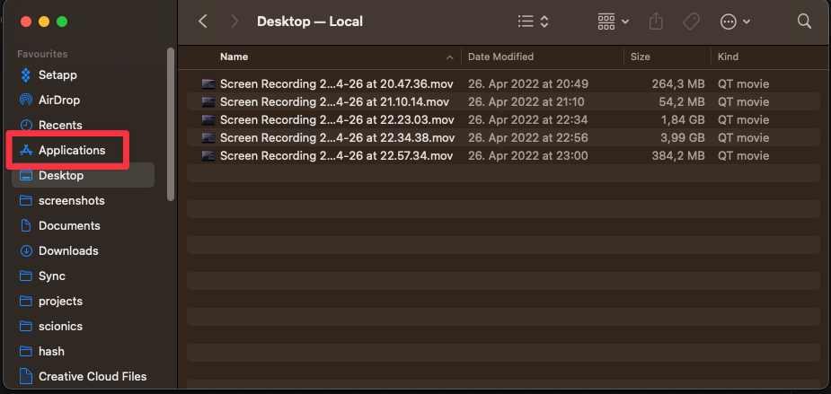
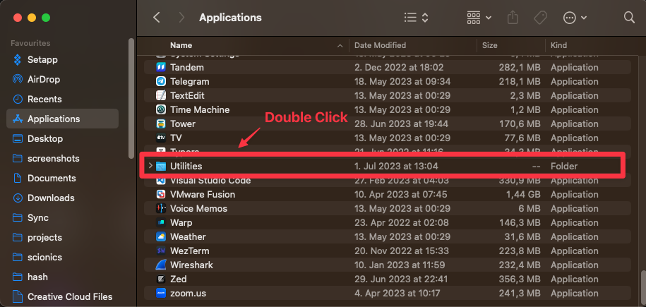
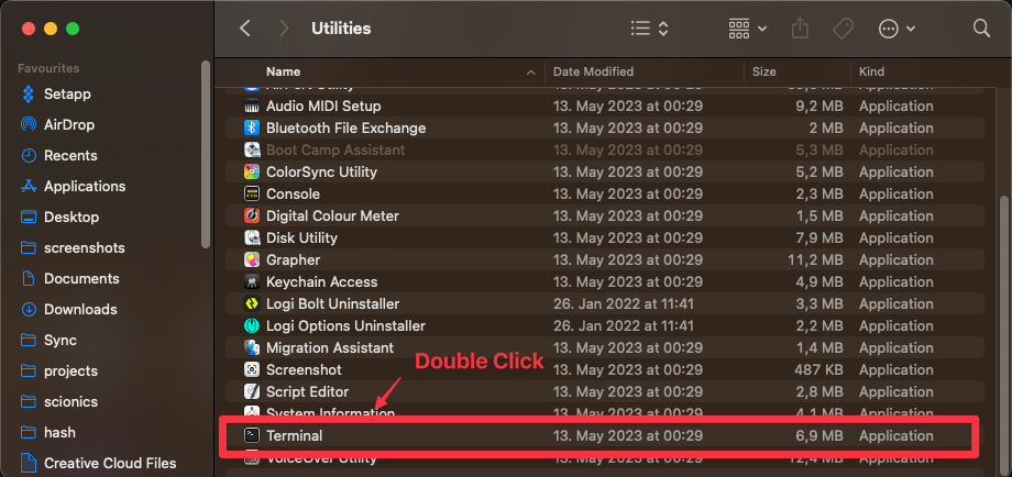
Navigating the Terminal

Changing Directories

You can change directories by using the cd command. (cd stands for change directory)

cd <path>

The <path> can be either an absolute path or a relative path.

Listing Files

You can list the files in your current directory by using the ls command. (ls stands for list)

ls

You can also list the files in a different directory by specifying the directory as an argument.

ls <path>

ls has several options that can be used to change its behavior, these include:

• -a - Show all files, including hidden files. (a stands for all)
• -l - Show the long format of the files. (l stands for long)
• -h - Show the file sizes in human readable format. (h stands for human readable)

You can combine these options, for example to show all files in the long format you can use ls -al.

Note: I recommend using ls -lah as your default ls command.

Creating Directories

You can create directories by using the mkdir command. (mkdir stands for make directory)

mkdir <path>

This will error out if the directory already exists, or you don't have the permissions to create the directory.

To create a nested directory structure you can use the -p option. (p stands for parents)

mkdir -p <path>

This will create all the directories in the path that don't already exist.

Removing Directories

You can remove directories by using the rmdir command. (rmdir stands for remove directory)

rmdir <path>

This will only remove the directory if it is empty.

Note: This command is seldom used, as it is often more convenient to use rm -rf.

Copying Files

You can copy files by using the cp command. (cp stands for copy)

cp <source> <destination>

You can also copy directories by using the -r option. (r stands for recursive)

cp -r <source> <destination>

Moving Files and Directories

You can move files and directories by using the mv command. (mv stands for move)

mv <source> <destination>

To rename a file or directory, you also use the mv command.

mv <original-name> <new-name>

This will error out if the destination already exists, or you don't have the permissions to move the file or directory.

Removing Files and Directories

You can remove files and directories by using the rm command. (rm stands for remove)

rm <path>

You can also remove directories by using the -r option. (r stands for recursive)

rm -r <path>

This will ask for confirmation if you are trying to remove a directory, to skip the confirmation you can use the -f option. (f stands for force)

rm -rf <path>

Note: This command is very dangerous, as it will remove the directory and all its contents without asking for confirmation. Double check that you are removing the correct directory before running this command.

This will error out if the file or directory doesn't exist, or you don't have the permissions to remove the file or directory.

Creating Files

You can create files by using the touch command.

touch <path>

This will create an empty file at the specified path.

Opening Files

You can open files by using the open command.

open <path>

This will open the file with the default application for that file type.

Printing Files

You can print files by using the cat command. (cat stands for catenate)

cat <path>

This will print the contents of the file to the terminal.

Searching Files

You can search files by using the grep command. (grep stands for global regular expression print)

grep <pattern> <path>

This will print all the lines in the file that match the specified pattern.

Finding Files

You can find files by using the find command.

find <path> -name <pattern>

This will print all the files in the specified path that match the specified pattern.

Editing Files

You can edit files by using the nano command.

nano <path>

This will open the file in the nano text editor. There are a multitude of other text editors available, but nano is the easiest to use.

To open a file in VSCode you can use the code command.

code <path>

Current Working Directory

You can print the current working directory by using the pwd command. (pwd stands for print working d irectory)

pwd

Interacting with Python

Python has two modes of operation, interactive mode and script mode.

Interactive Mode

You can start Python in interactive mode by running the python command.

python

This will start the Python REPL (Read-Eval-Print-Loop), which is a program that reads Python code, evaluates it, prints the result, and then loops back to read the next line of code.

This mode is useful for testing out small snippets of code, but is not suitable for writing large programs. Nothing you do in interactive mode will be saved, so you will have to retype everything the next time you start Python.

To exit the Python REPL you can use the exit() function (or press Ctrl+D)

exit()

Script Mode

You can run Python scripts by using the python command.

python <path>

This will run the Python script at the specified path.

Git Cheat Sheet

Further Reading